你的位置：首页 > 读后感 > 文章正文

Intro to RL Chapter 3: Finite Markov Decision Process

时间: 2021-04-10 16:50:16 | 作者：斑马 | 来源: 喜蛋文章网 | 编辑: admin | 阅读: 105次

在MDP中，action不仅影响immediate reward，也影响未来的reward。

3.1 The Agent-Environment Interface

Dynamics of finite MDP: $p(s^prime, r leftvertright. s, a) = Pr{S_t ` s^prime, R_t = r leftvertright. S_{t-1} = s, A_{t-1} = a} tag{3.2}$ 根据3.2，我们可以计算state-transition probabilities p(s^prime leftvertright. s, a)

，expected reward given state and reward r(s, a)

，expected reward for state-action-next-state r(s, a, s^prime)

。RL问题中，state、action的选择更多是art而非science

3.2 Goals and Rewards

reward指明goal，但是不能给agent prior knowledge，比如下围棋，赢了一局给1分，但是agent并不知道该怎么下。what you want it to achieve, not how you want it achieved。

3.3 Returns and Episodes

episodic tasks：有terminal states，cumulative reward直接加起来就好。continuing tasks：更多RL问题没有terminal states，一直跑啊跑啊跑啊，于是用discounting来计算discounted return， gamma

为discounted rate： $G_t = R_{t+1} + gamma R_{t+2} + dots = sum^infty_{k=0} gamma^k R_{t+k+1}. tag{3.8}$ 若 gamma < 1

，只要 ${R_k}$ 有限制，则3.8式为finite value；若 gamma = 0

，则只考虑immediate reward。 $begin{align} G_t &= R_{t+1} + gamma R_{t+2} + gamma ^ 2 R_{t+3} + dots &= R_{t+1} + gamma (R_{t+2} + gamma R_{t+3} + dots) & = R_{t+1} + gamma G_{t+1}. end{align} tag{3.9}$ 只要 gamma < 1

，3.8就是finite $sum^infty _{k=0} gamma ^ k = frac{1}{1-gamma} tag{3.10}$

3.4 Unified Notation for Episodic and Continuing Tasks

用abosorbing state 将episodic tasks 和continuing tasks结合，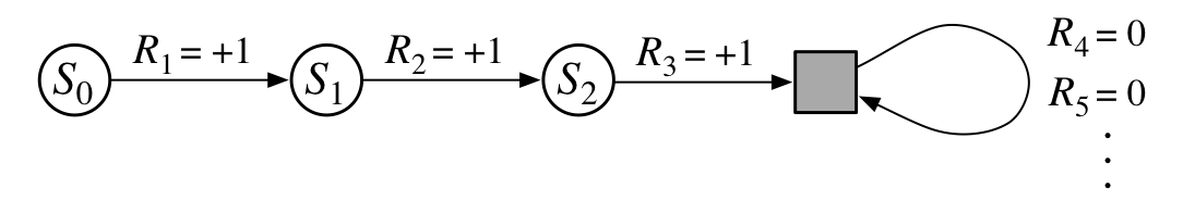

于是episodic tasks的reward变成 $G_t = sum ^T_{k=t+1} gamma ^{k-t-1} R_k$ ， T = infty

（or both）。

3.5 Policies and Value Functions

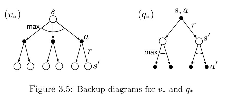
value function: how good it is for the agent to be in a given state (or how good it is to perform a given action in a given state).policy pi (a leftvertright.s)

: a mapping from states to probabilities of selecting each possible action.The value of a state

under a policy

, denoted

, state-value function for policy

: $v_pi (s) = mathbb{E} _pi [G_t leftvertright. S_t = s] = mathbb{E} _pi [sum^{infty} _{k=0} gamma ^k R_{t+k+1} leftvertright. S_t = s], text{ for all } s in S. tag{3.12}$ action-value function for policy : $q_pi (s, a) = mathbb{E}_pi [G_t leftvertright. S_t = s, A_t = a] = mathbb{E}_pi [sum^infty_{k=0} gamma^k R_{t+k+1} leftvertright. S_t=s, A_t=a]. tag{3.13}$ Monte Carlo methods：把所有可能都试了，计算average。也可以用parameterized functions来表示 v_pi, a_pi

，不断调整参数。虽然依赖于approximator，但也可以听精确。在value function 中，有Bellman equation成立，是很多计算value function的基础： $begin{align} v_pi (s) &= mathbb{E} _pi [G_t leftvertright. S_t = s] &= mathbb{E}_pi [R_{t+1} + gamma G_{t+1} leftvertright. S_t=s] &= sum_a pi(a leftvertright. s) sum_{s^prime}sum_{r} p(s^prime, r leftvertright. s, a)[r+gamma mathbb{E}_pi [G_{t+1} leftvertright. S_{t+1} = s^prime]] &= sum_a pi(a leftvertright. s) sum_{s^prime, r} p(s^prime, r leftvertright. s, a) [r+gamma v_pi (s^prime)], text{ for all } s in S. end{align} tag{3.14}$

3.6 Optimal Policies and Optimal Value Functions

$pi geq pi^prime text{ if and only if } s_pi (s) geq v_{pi^prime} (s) text{ for all } s in S.$ 总存在一个policy优于其他policy或相等，称为optimal policy pi_*

。所有的optimal policies 有相同的state-value function，称为optimal state-value function v_*(s)

，相同的optimal action-value funtion q_*(s)

。

无需指定policy（independent of policies），直接取max就可。Bellman optimality equation： $v_*(s) = max_a sum_{s^prime, r} p(s^prime, r leftvertright. s, a)[r+gamma v_*(s+1)]. tag{3.19}$ q_*(s, a)